Optical QPSK

Basic conditions

The difference to the electrical QPSK is that an adder is used instead of a multiplier!
The basic brightness is the reason that an offset occurs in the photodiode!

This simulation shows how an optical QPSK with an external modulator and a direct conversion receiver works. A 10 GBit/s connection is established at 1500 nm.

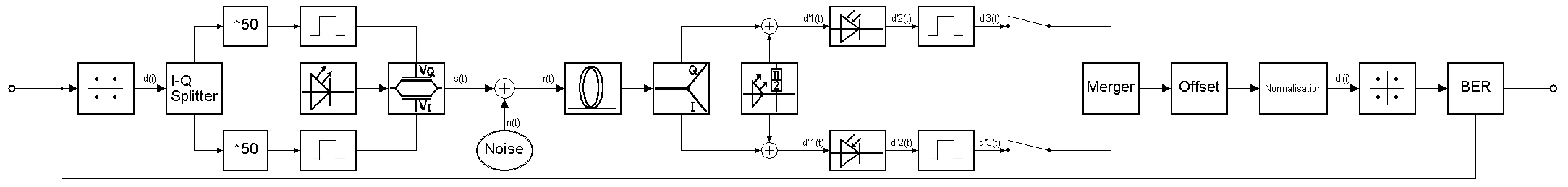
The optical transmission consists of an electrical signal that, with the help of a modulator, is converted into an optical signal.
Afterwards the signal is sent through an optical fiber to the receiver, where it's demodulated and reverted into an electrical signal by using a photodiode.

The carrier signal of the direct conversion receiver and the received signal should be synchronized in frequency and phase.
In real life optical QPSK requires a subsequent phase correction.

To simplify and to help with a better understanding of the simulation the following points will be ignored:

- the phase shift of all the different components
- the influence of temperature
- non-ideal lasers (they will have an exact wavelength and phase)

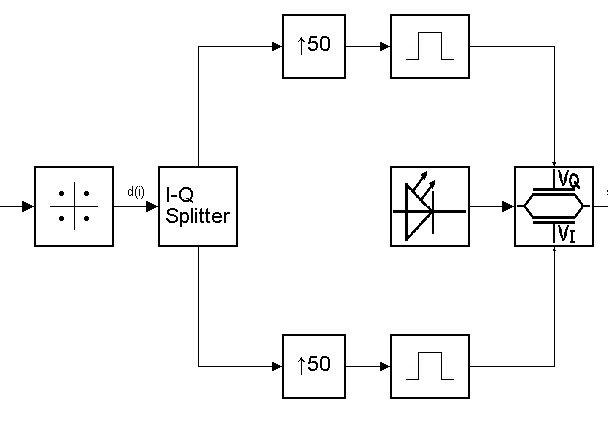
Modulation

It consists of a modulation symbol mapper, an I/Q splitter, a pulse shaper for the I and Q path, a local laser and a 'Mach-Zehnder-Interferometer'.
For further information refer to Mach-Zehnder-Interferometer.

$LiNb{O}_3$ , Lithium niobate a synthetic salt, is used as a phase shifter.
(At this point there is no use to get into the chemical componets of the synthetic salt, just know that it helps with shifting the phase.)
The signal goes to the I/Q splitter, there it gets separated into the I and Q path.
Afterwards the pulse shaper on both paths of the 'Mach-Zehnder-Interferometer' feeds the signal into the local laser.

The phase shift can be calculated with the formula below:

$$\phi =\frac{{\omega }_{0}L\Delta n_{eff}}{c}$$

The phase shift in the Q path can be either 90° or 270°, in the I path 0° or 180°.
At the end of the 'Mach-Zehnder-Interferometer' both paths are added resulting in four phase shifts (±45° and ±135°).
The following signal goes to the optical fiber.

❮ ❯

TRANSMISSION ATTENUATION

The transmission attenuation of the optical fiber is calculated from the length and the attenuation per kilometer.
Moreover an additional attenuation can be added, for example as a bend.
A further requirement is the addition of AWGN.

$$S_r=S_t·a^2=\frac{{\hat{r}}^2}{2}\Rightarrow \hat{r}=\sqrt{2S_t}·a$$

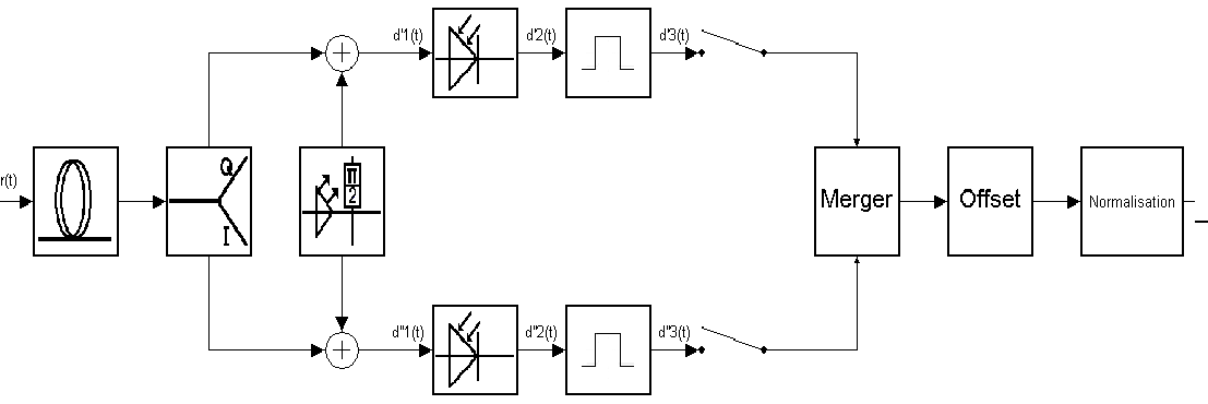
DEMODULATION

To demodulate the signal it has to be split into two paths.
Both paths add a local laser, one of them getting a 90°, the other a 0° phase shift.
Afterwards the signals are sent to two photodiodes, where they are converted into electrical signals.
Subsequently there is an electrical Q- and I-signal. Both will be combined to form a constellation point.

>

For a better understanding regarding how the signals get processed and how the formulas get derived, read the first part of the tab: illustration.

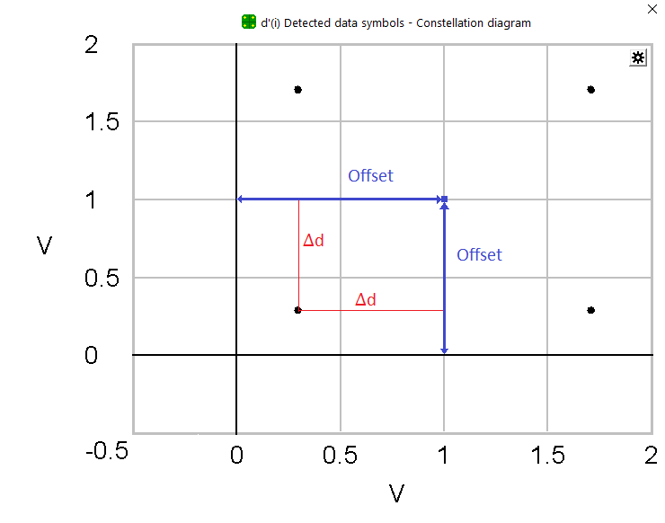
OFFSET CORRECTION

The photodiode is a power detector and since light can't have a negative amplitude it produces only positive output values.
As a consequence, the constellation is shifted to the fist quadrant.
Zero, as the lowest point, exists only if the local laser and the received signal eliminate each other completely.
But keep in mind that the offset is the same for Inphase as in Quadrature!
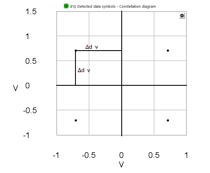
Therefore offset correction is used to center the constellation.

Offset correction, explained in short terms, can be seen as the mean of the signal.
To get a better grip on the finer details, read the relevant part of the tab: illustration.

Constellation diagram with offset

Constellation diagram with offset correction

Experiment

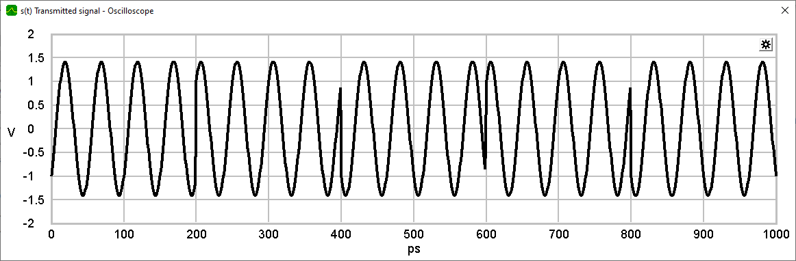
As part of the experiment, the frequency is kept low so that it can be displayed.

In order to show how optical QPSK works, the following experiment will be performed.

PART 1

The aim is to have the received signals have the same value, and the constellation points are on $\frac{\sqrt{2}}{2}$.

Explore the signal values at all points mentioned in the tutorial to get acquainted with the process.
Try to understand how the offset correction, set in the application, results from the calculation explained in the illustration.

After having read the tutorial, and understand the formulas and change the length of the optical fiber to 120 km and the attenuation to 0.3 dB/km.
For simplicity reasons change the noise setting to 'OFF'.
The default settings are shown in the folder 'Manual'.

Calculate the new values of the offset correction and check your result with the constellation diagram.

PART 2

As soon as the previous steps have been understood, the second part can start.
Switch back to the 30dB-channel (optical fiber length: 150km, attention: 0,2dB).

Alter the noise setting to 'ON' and change the SNR bit by bit in favor to get the same BER values as in the table below.
Tip: Changing the SNR results in another offset. So it´s recommended to make an Excel-sheet for the calculation.
Are these the exact same values? If not, how and why do they differ?
For further understanding compare the optical to the electrical QPSK.

Simulation Settings

The simulation starts with the following default settings.
Those can be changed by pressing the respective icons.

Simulation settings:

transmit laser:1V

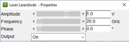laser diode properties

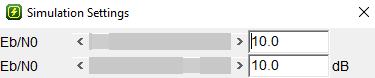simulation settings ($E_0/N_b$ ):10dB

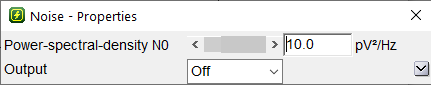noise properties result of simulation settings

transmission attenuation: 30dB(150km, 0,2dB/km)

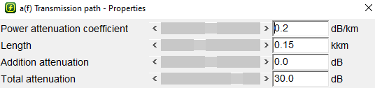transmission path properties

local laser:1V

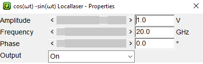local laser properties

photodiode

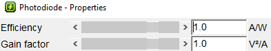photodiode properties

offset:-0,5V

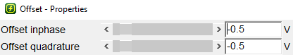offset properties

normalization:30

normalization properties

Demodulation - Formulas explained

The local laser has the following characteristics:
$\hat{c} = 1V; \frac{{{\displaystyle \hat{c}}}^2}{2} 0.5V^2 \Rightarrow dBm = dBm{V}^2$

Optical demodulation differs from the electrical one in that, that the carrier signal is added instead of multiplied.
Below the formulas are explained, which will be used to calculate the signals $d$₁(t) , $d$₂(t) , $d$₃(t) .
The signal after the optical coupler: $d$₁(t) .
The signal after the photodiode: $d$₂(t) .

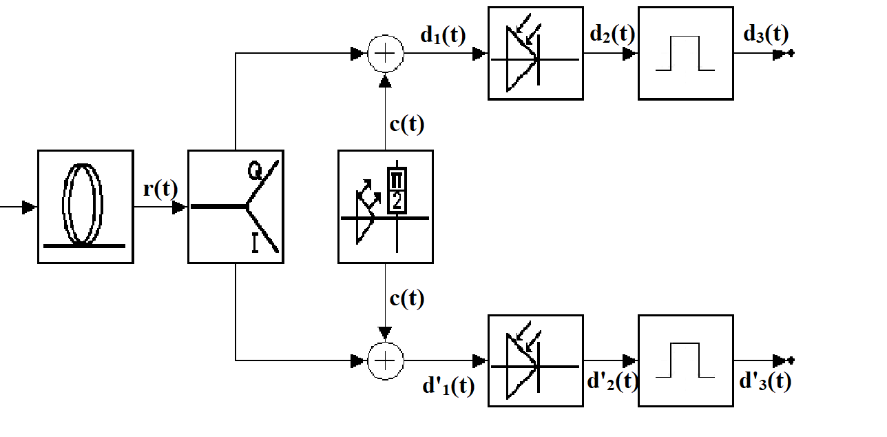
QPSK Demodulator

First the mean of r(t) has to be calculated, since the signal splits into two paths (as shown in the graphic). Then it will be added to the carrier signal c(t). $d_1\left(t\right)=\frac{\hat{r}}{\sqrt{2}}\cos ({\omega }_{0}t+{\phi }_r)+\hat{c}\cos ({\omega }_{0}t+{\phi }_c)$ In the next step the photodiode squares $d$1(t) . $d_2\left(t\right)=(d_1{\left(t\right))}^2=(\frac{\hat{r}}{\sqrt{2}}\cos ({\omega }_{0}t+{\phi }_r)+\hat{c}\cos {({\omega }_{0}t+{\phi }_c))}^2$ The first binomial formula can be used to simplify the term. ${(x+y)}^2=x^2+2xy+y^2$ $=\frac{{\hat{r}}^2}{2}\cos ({\omega }_{0}t+{\phi }_r{)}^2+{\hat{c}}^2\cos ({\omega }_{0}t+{\phi }_c{)}^2+2\frac{\hat{r}\hat{c}}{\sqrt{2}}\cos ({\omega }_{0}t+{\phi }_r)·\cos ({\omega }_{0}t+{\phi }_c)$ The pulse shaper generates the average, which results in the detected signal $d$3(t) . It consists of the Offset and $∆d$, the shift of the signal. Reminder: ${\cos }^{2}x=\frac{1}{2}(1+\cos 2x)$ and Going forward, the cosine-parts of the formula can be discarded. $d_3\left(t\right)=\frac{{\hat{r}}^2}{4}+\frac{{\hat{c}}^2}{2}+\frac{2\hat{r}\hat{c}}{\sqrt{2}}*\frac{\sqrt{2}}{4}$ The blue part causes an offset, while the red part equals to $∆d$ For clarification: $\frac{\sqrt{2}}{4}$ consists of $\frac{1}{2}$ from the cosine theorem above and the 45° displacement in the constellation diagram $\frac{1}{2}\sqrt{2}=\frac{\sqrt{2}}{2}$ To finish the formula, the Noise needs to be added, but don't forget to divide it by 2, since it splits into two paths. $d_3\left(t\right)=\frac{N}{2}+\frac{{\hat{r}}^2}{4}+\frac{{\hat{c}}^2}{2}+\frac{2\hat{r}\hat{c}}{\sqrt{2}}*\frac{\sqrt{2}}{4}$

Offset Correction - Formulas explained

Offset correction is based on the mathematical formula of the detected power.
Below the two components of the formula $d$₃(t) , as derived above, are being used to calculate them respectively.

$Offset=\frac{Na²}{2}+\frac{{\hat{r}}^2}{4}+\frac{{\hat{c}}^2}{2}=\frac{(S_t+N)a^2}{2}+\frac{{\hat{c}}^2}{2}$

a is the damping factor and has to be multiplied to the noise. r is the received amplitude and can be expressed with the transmission power.
$r=\sqrt{2S_t}a$

Furthermore r has to be squared to fit into the formula.
$\frac{2N{a}^2}{4}+\frac{2S_t{a}^2}{4}=\frac{2(N+S_t)a^2}{4}$
The last step, to get to the finished Offset formula, is to shorten the four with the two.

$∆d=\frac{2\hat{r}\hat{c}}{\sqrt{2}}\frac{\sqrt{2}}{4}=\frac{\hat{r}\hat{c}}{2}=\frac{\sqrt{2S_t}a\hat{c}}{2}$

Here $△d$ only requires shortening and replacing the r with the formula mentioned above.

The final step requires a factor v, which describes multiplied with $△d$ the corrected position of the constellation points in the diagramm, as shown below.

Constellation diagram with offset

Constellation diagram with offset correction

The desired position in the constellation diagram is at 45° from zero, so both values multiplied should result in $\frac{1}{2}\sqrt{2}$, which is also the value of $\cos (45°)$.

$v·∆d=\frac{\sqrt{2}}{2}\Rightarrow v·\frac{\sqrt{2S_t}a\hat{c}}{2}=\frac{\sqrt{2}}{2}\Rightarrow v=\frac{2}{\sqrt{S_t}2a\hat{c}}$