Interactive simulation of communication systems
On this site experiments in the field of communications technology are provided online free for use.
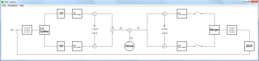
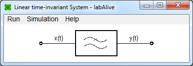
Each experiment uses a specific simulation that is implemented using labAlive. labAlive is a graphical and interactive simulator tool for communications systems. The virtual experiment environment emulates a real-world laboratory.
- Intuitive tool
- Mediator between theory and practice
- Teaching aid
 |
 |
 |
 |
 |
 |
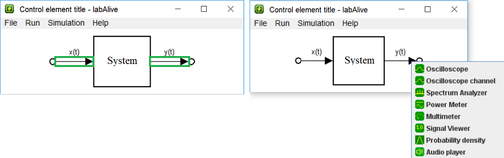
Open measures and system properties
| Click on wire | Open measure |
|---|---|
Left click on a wire.  |
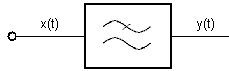
Open the default measure, usually oscilloscope.
|
Right click on a wire.
|
Select a measure. The set of offered measures depends on the signal type of the wire, e.g. analog, digital, complex signal.
|
| Click on system | Open system properties |
|---|---|
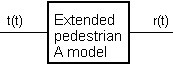
Left click on a system box or a bullet representing a generator.
|
 |
Right click on a system box.
|
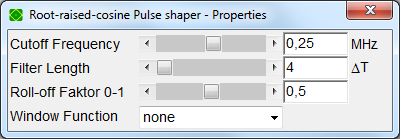
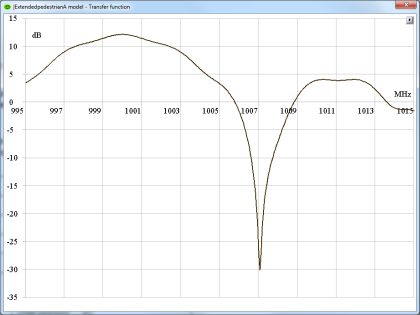
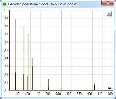
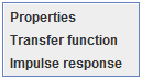
View the transfer function or impulse response of filters.
|
Measure settings
Click on the settings icon to adjust instrument settings.Click on settings icon  |
Open measure settings |
|---|---|
|
|
|
|
Click on more details button  |
Open measure settings details |
|---|---|
|
|
|
|
|
|
Menu
| Menu | Action |
|---|---|
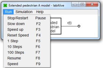 |
Pause, continue and control speed of the simulation. |
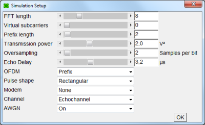 |
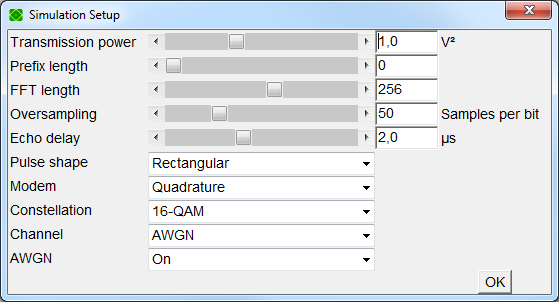
Modify the setup and restart the simulation. |
Keys & shortcuts
| Key | Action |
|---|---|
| Pause | Pause or continue the simulation. |
| F2 | Slow down the simulation speed (50%). |
| F3 | Speed up the simulation speed (200%). |
| F4 | Reset to initial simulation speed. |
| 1 | Process one simulation step and then pause. |
| 2 | Process 10 simulation steps and then pause. |
| 3 | Process 100 simulation steps and then pause. |
| 4 | Process 1000 simulation steps and then pause. |
| 5 | Process 10000 simulation steps and then pause. |
| 6 | Process 100000 simulation steps and then pause. |
| F8 | Show speed slider.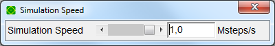 |
| F9 | Show simulation status.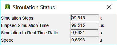 |
| F10 | Show preferences dialog.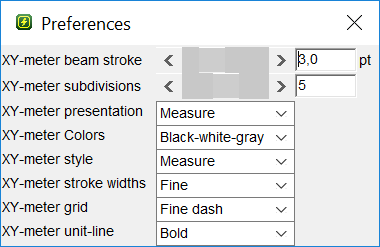 |
| F11 | Show simulation settings dialog. (Depends on simulation)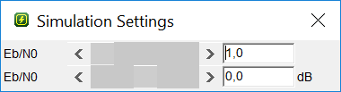 |
| F12 | Show simulation setup dialog. (Depends on simulation)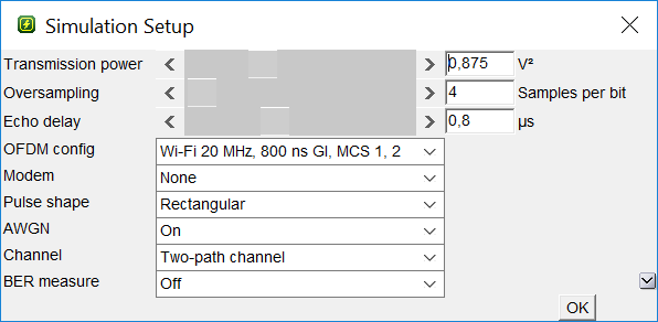 |
Measures overview
With mylabAlive you can simulate so many different hardware experiments that the range of possibilities are up to yourself. You'll need different measures to see or hear what the simulation is doing.
Each measure is designed for a special field. The best thing is, the instruments would cost a lot in reality, but are free in these simulations.
| Name | Code |
|---|---|
| Audio Player | audioPlayer |
| Audio Player Stereo | audioPlayerStereo |
| ComplexScope | complexScope |
| Constellation Diagram | constellationDiagram |
| Digital Oscilloscope | digitalScope |
| Multimeter | multimeter |
| Oscilloscope | scope |
| Oscilloscope, ImpulseResponse | impulseResponseScope |
| Powermeter | powermeter |
| Probability Density | density |
| Signal Logging | signalLogging |
| Signal Viewer | signalViewer |
| Spectrumanalyzer | spectrum |
| Spectrumanalyzer, Transferfunction | transferFunctionSpectrum |
| TransmitchainSignalLabels | transmitChainSignalLabels |
| XY Meter | xyMeter |
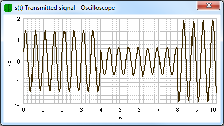
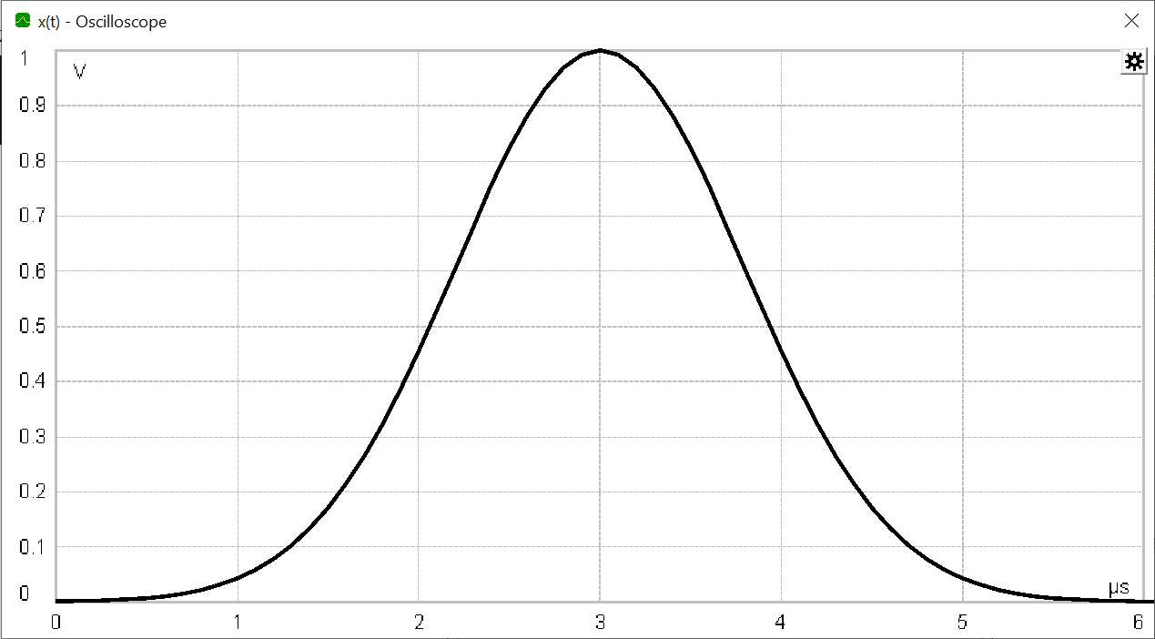
Oscilloscope - operate and control
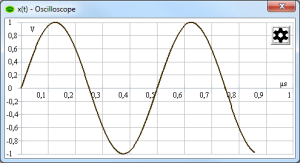
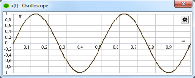
The oscilloscope is one of the most important/significant measuring instrument in electronics. This description is designed to give an overview about the measure.
Open oscilloscope
Depending on the simulation, the oscilloscope opens automatically. Alternating open the scope by right-click on the wire and selecting oscilloscope. Left-click on the wire will open the default measure, which is also usually the oscilloscope.

In some simulations the scope will start togehter with the control element. Depending on the experiment, the scope may differ in form of the background, beam and grid. To get more informations about these design settings, please visit the Preferences tab.
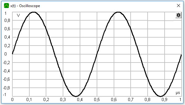
Measure
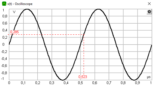
To measure the amplitude of the signal at a certain time or measure the rising time of a signal to a certain amplitude, mark the signal by clicking at the spot with the left mouse. A fine red-dotted line shows the time and amplitude at the marked spot.
The marked measuringspot will dissappear within the next cycle of the oscilloscope. To prevent this, press Pause on the keyboard to pause the simulation. After the simulation pauses, the measuringspot will stay at the display. To restart the simulation, again press the Pause key.
To delete the marker, double-click with the left mouse on the scope and the marker disappear.
Open settings
We discussed how to change the design of the scope. If you want to change the amplitude/ division, time/division or shift the signal you can open the settings menu with 2 options.
First method: Right-click on scope
The menu will popup and display all settings (Picture 4).
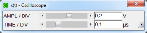
Second method: Gear symbol
Click on the gear symbol located in the upper right corner of the scope. The ampl/div and time/div settings appear. With the arrow on the right-side (green circle), you can open further adjustments.
Note: You need to click through 2 more stages to get to the full settings menu.
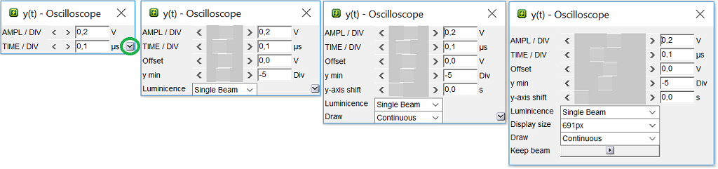
In picture 4 you can see the settings menu. Declaration of every single setting can be found in table 1.
| Settings | ||
|---|---|---|
| AMPL / DIV | Changes the amplitude per division. Affects the y-axis |  |
| TIME / DIV | Changes the time per division. Affects the x-axis |  |
| Offset | Adds a certain offset of the signal. Affects the y-axis |  |
| y min | Shifts the zero-line horizontally. |  |
| y-axis shift | Shifts the y-axis vertical. | |
| Draw | Continous Discrete Dirac Sample & hold |
 |
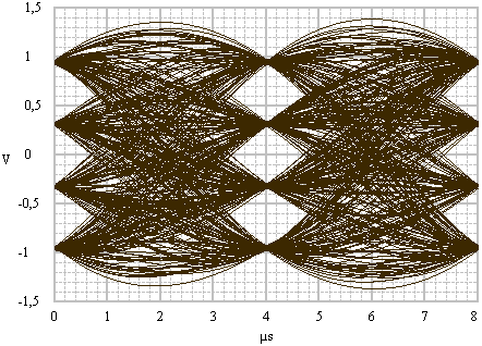
| Luminiscence | Single beam Luminiscence Eye pattern |
|
| Display size | Frame - half 441px Frame - quarter 219px Frame - full 890px Diagram - quarter 219px Diagram - half 441px Diagram - full 890px Print - quarter 477px Print - half 943px Print - full 1906px 604px |
|
| Keep Beam | Freezes the the graph | |
Copy paste signal
The oscilloscope can also show more than one beam at a time.
Simply select the window from which you want to copy the
beam and press "Ctrl + C".
Change to your desired oscilloscope window and press "Ctrl + V".
Now a new colored beam should appear.
Note: If you resize the window only the original signal will remain.
Picture 5: Oscilloscope before copy |
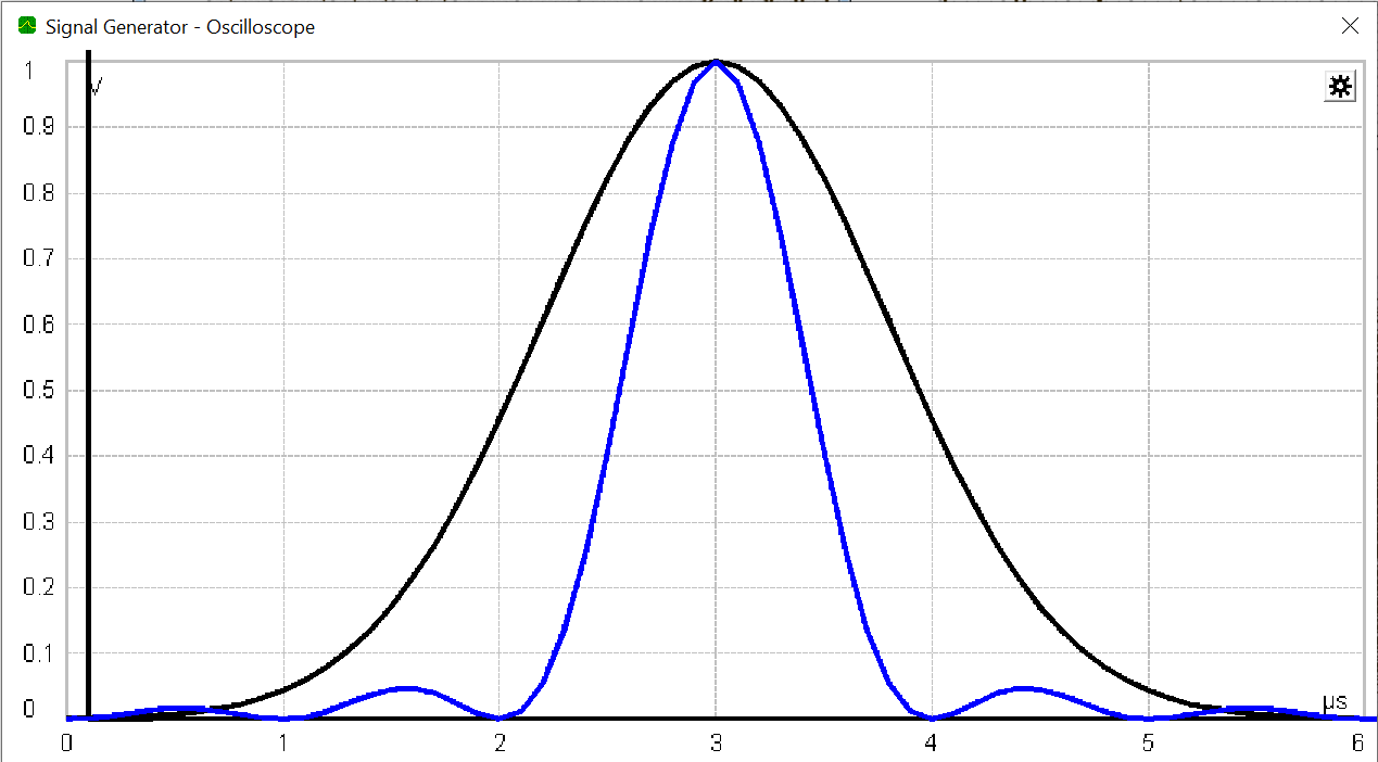
Picture 6: Oscilloscope after paste |
Other Oscilloscopes
| Measure | Code |
|---|---|
| ComplexScope | complexScope |
| digital oscilloscope | digitalScope |
| oscilloscope, impulseresponse | impulseResponseScope |
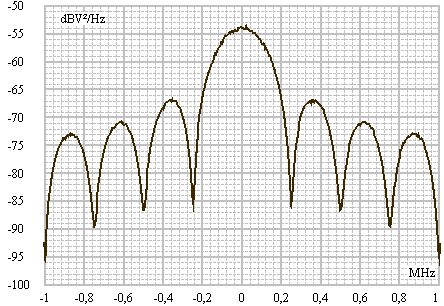
Spectrum analyzer - operate and control
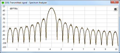
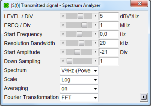
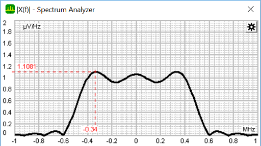
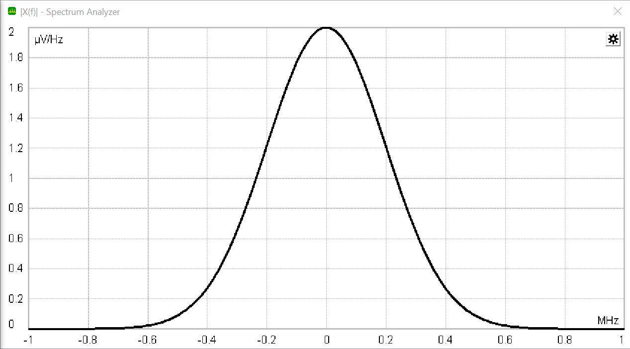
Next to the oscilloscope(put link in here), the spectrum analyzer is an important instrument in the development of circuits. A spectrum analyzer is a piece of electronic equipment that is used to measure the magnitude of an input signal set against the full frequency range of the instrument. The x axis shows the frequency and on the y axis the amplitude/level.
Open spectrum analyzer
Note, whether the simulation automatically opens the spectrum analyzer, you are able to open the measure by right-click on the wire and selecting Spectrum Analyzer
In some simulations the spectrum analyzer will start togehter with the main window. Depending on the experiment, the display may differ in form of the background, beam and grid. To get more informations about the settings, please visit the Preferences tab.
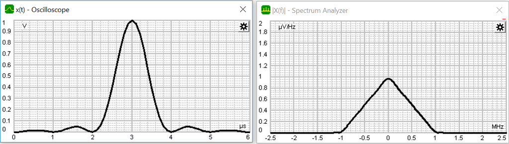
Measure
The spectrum analyzer can be used to measure the amplitude/level at a certain frequency. Mark the frequency with the left mouse button. A fine, red-dotted line shows the frequency and amplitude/level at the marked spot.
To delete the marker, double-click with the left mouse button on the scope. The marker disappear.
Open settings
To change the amplitude/division, time/division or shift the signal open the settings menu with one of the 2 following options.
First method: Right-click on scope
The menu will popup and display all settings (Picture 4).
Second method: Gear symbol
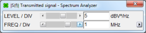
Click on the gear symbol located in the upper right corner of the scope. The ampl/div and time/div settings appear. With the arrow on the right-side (green circle), you can open further adjustments.
Note: You need to click through 2 more stages to get to the full settings menu.
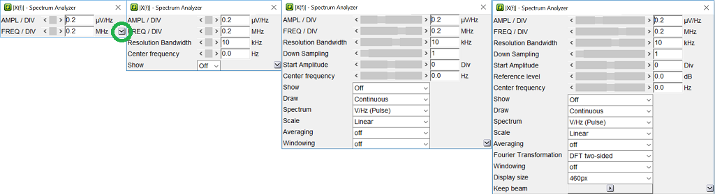
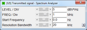
In picture 4 you can see the settings menu. Declaration of every single setting can be found in table 1.
| Settings | ||
|---|---|---|
| AMPL / DIV | Changes the amplitude per division. Affects the x-axis |  |
| FREQ / DIV | Changes the frequency per division. Affects the y-axis |  |
| Resolution Bandwidth |  |
|
| Down Sampling | ||
| Start Amplitude | Adds/subtracs Divisions |  |
| Reference level | Sets the reference level |  |
| Center Frequency | Changes the start frequency (Only TransferFunction Spectrum) |  |
| Start Frequency | Changes the start frequency |  |
| Draw | Continous Discrete Dirac Sample& hold |
 |
| Spectrum | V(Periodical) V/Hz(Pulse) V²/Hz(Power density) (Transfer Function) |
|
| Scale | Linear Log |
|
| Averaging | On Off |
|
| Fourier Transformation | FFT DFT DFT two-sided |
|
| Windowing | Off On |
|
| Display size |
Frame - half 441px Frame - quarter 219px Frame - full 890px Diagram - quarter 219px Diagram - half 441px Diagram - full 890px Print - quarter 477px Print - half 943px Print - full 1906px 604px |
|
| Keep Beam | Freezes the the graph | |
Copy paste signal
The spectrum analyzer can also show more than one beam at a time.
Simply select the window from which you want to copy the
beam and press "Ctrl + C".
Change to your desired spectrum analyzer window and press "Ctrl + V".
Now a new colored beam should appear.
Note: If you resize the window only the last copied signal will remain in addition to the original signal.
Picture 5: Spectrum analyser before copy |
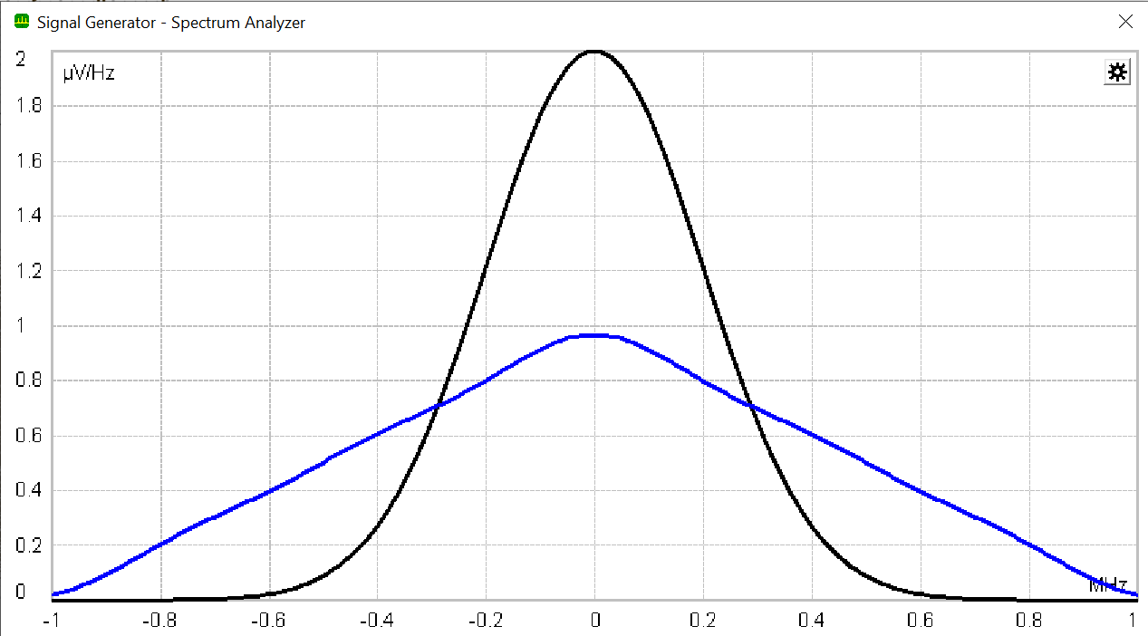
Picture 6: Spectrum analyzer after paste |
Other spectrumanalyzer
| Measure | Code |
|---|---|
| Spectrumanalyzer, transferfunction | transferFunctionSpectrum |
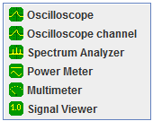
Small Measures
labAlive provides additional small measures which allows the user to perform a large number of different measurements. Each measure covers a specific field of measurement. This overview is designed to show each measure with an image of the interface, a small introduction and a table with the corresponding code.
To use one of the measure in a simulation, take the code from the corresponding table and paste it into the sourcecode of the simulation.
Multimeter
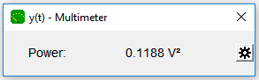
The multimeter is an electronic measure that combines several measurement functions in one unit. Against the "real" multimeter this one can measure power, average of the signal, PAPR and peak amplitude.
To change the measure function, click on the gear symbol located on the right side of the GUI. Table 1 shows an overview of all functions.
| Multimeter | ||
|---|---|---|
| Mode | Unit | Description |
| Power | V² | Normalized electric instantaneous power |
| Average | V | Arithmetic mean of the signal |
| Peak-to-average power ratio | dB | PAPR is the peak amplitude squared (peak power) divided by the average power |
| Peak amplitude | V | Peak amplitude of the signal |
The measure can be called in the source code of the simulation. To include this, please consider to take the code out of table 2.
| System | Code |
|---|---|
| Multimeter | multimeter |
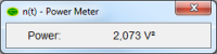
Power Meter
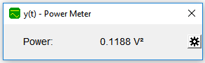
A power meter ist a electronic measure that measures the amount of electric energy. In this case, the power meter measures the energy of signals in V². This is the only measurement function.
The measure can be called in the source code of the simulation. To include this, please consider to take the code out of table 3
| System | Code |
|---|---|
| Power Meter | powerMeter |
Signal viewer
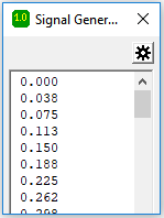
The signal viewer is a tool which allows the user to see the current value of the signal. This device measures voltages in V and prints the value in a decimal number.
The signal viewer prints the value on the screen. The values can be logged with the signal logging tool.
These measures can be called in the source code of the simulation. To include this, please consider to take the code out of table 4.
| System | Code |
|---|---|
| Signal viewer | signalViewer |
| Signal logging | signalLogging |
Audio player
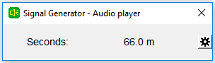
The audio player can be used to play the signal like an audio wave.
These measures can be called in the source code of the simulation. To include this, please consider to take the code out of table 5.
| System | Code |
|---|---|
| Audio player | audioPlayer |
| Audio Player Stereo | audioPlayerStereo |
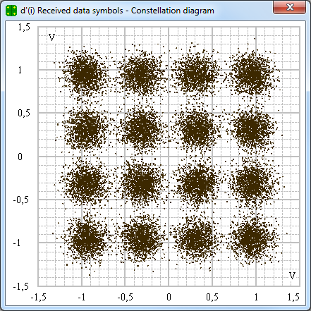
Constellation diagram
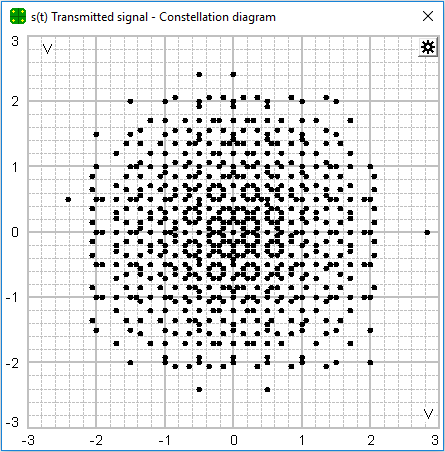
A constellation diagram displays the signal as a two-dimensional xy-diagram. The angle of each point represents the phase shift of the carrier wave. Most times this tool is used together with QPSK and PSK applications.
The measure can be called in the source code of the simulation. To include this, please consider to take the code out of table 6.
| System | Code |
|---|---|
| Constellation diagram | constellationDiagram |
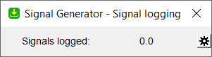
Signal logging
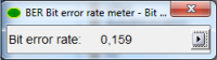
There is a signal logging function available. It can be used to save samples in multiple file formats. To use it, right click on the connection that you want to log and choose "Signal logging". The following window will open. It shows the current amount of logged samples.
By clicking on the gear symbol on the right of the new window, you can set up the signal logger for proper use. A new window will be opened.
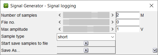
| Field | Description | Example |
|---|---|---|
| Numbers of samples | With this options it is possible to set the number of samples to be saved to the sample-file. | 2 M -> 2 million samples will be saved |
| File no. | Sets the number, that will be appended to the standard filename. | standard filename: "samples_<File no.>.<sampletype>a" |
| Max amplitude | This only applies to the sample types short and wave. It is used for setting the allowed range of voltages for the samples. | 1.3V |
| Sample type | Sets the file format, the data will be stored in. | short, float, double, wav |
| Start save samples to file | Starts the process of saving samples to a file. | |
| Save As... | Opens a location-chooser window. If not specified, samples will be saved to a sub folder in the users home directory. It works on a variety of operating systems. | standard location on Windows: C:\Users\<User-Name>\ labAlive\samples\ |